Wetlands cover between 3% and 8% of the Earth’s land surface and provide ecosystem services disproportionate to their extent: flood attenuation, water quality improvement, carbon sequestration, and biodiversity support (Mitsch and Gosselink, 2015; Davidson, 2014). Despite this, most countries lack comprehensive wetland inventories. Existing maps are fragmented, produced at incompatible scales with inconsistent methods, and rarely updated to reflect the dynamic character of wetland systems (Finlayson et al., 2018; Mahdianpari et al., 2019). In sub-Saharan Africa, the problem is acute. Many wetlands of continental significance function with limited mapping, and those that exist rely on single-date optical imagery that captures a snapshot rather than the seasonal and inter-annual variability that defines wetland function (Rebelo et al., 2009; Muro et al., 2016).
Remote sensing offers the spatial and temporal coverage that field surveys cannot match, and two decades of methodological development have produced a substantial toolkit for wetland mapping (Ozesmi and Bauer, 2002; Mahdavi et al., 2018). Yet accurate mapping of inland wetlands remains difficult. Shallow, turbid waters confound optical classification. Cloud cover obscures tropical wet seasons precisely when inundation is greatest. Emergent vegetation masks the water beneath it. Coloured dissolved organic matter, suspended sediment, and phytoplankton blooms alter spectral properties in ways that atmospheric correction algorithms handle poorly (Matthews, 2011; Ogashawara et al., 2017). Higher-resolution sensors introduce their own constraints in spectral coverage, radiometric sensitivity, and temporal frequency (Palmer et al., 2015; Kutser, 2012).
The concurrent availability of Sentinel-1 SAR and Sentinel-2 optical data since 2014, combined with the multi-decadal Landsat archive made freely available since 2008, now provides an unprecedented opportunity to address these limitations through multi-sensor time series analysis. Cloud computing platforms, particularly Google Earth Engine (GEE), have removed the computational barriers that previously made processing such large volumes of satellite imagery infeasible on conventional systems (Gorelick et al., 2017; Mahdianpari et al., 2019). These advances enable on-demand, large-scale wetland mapping that was not possible a decade ago.
Endorheic watersheds in Africa present a further challenge that is not merely technical but social. Their ecological and economic significance is mediated by human populations whose livelihoods track the water. Remote sensing provides essential spatial data (Eva and Lambin, 2000; Philippe and Karume, 2019), yet it captures neither the adaptive strategies of local resource users nor the political ecology that governs access to fluctuating resources (Yiran et al., 2012; Sulieman and Ahmed, 2013; Demichelis et al., 2023). Maps that are technically defensible remain ecologically and socially incomplete.
The spatial unit of this study is the basin, a term whose precise hydrological meaning the lake at its centre tends to obscure. A drainage basin, equivalently a catchment or watershed, is the whole area that drains to a common outlet, bounded by topography rather than by any water body within it. In an endorheic basin that outlet is internal: no channel reaches the sea, and water leaves only by evaporation and seepage from the terminal lakes and swamps where drainage gathers (Wang et al., 2018). Closed basins of this kind cover close to a fifth of the continental land surface, concentrate in arid and semi-arid regions, and are losing water storage worldwide (Wang et al., 2018). Lake Chilwa lies at the floor of one, a transboundary catchment of roughly 8,300 km² shared between Malawi and Mozambique (Kambombe et al., 2023), which we delineate from the terrain rather than adopt from a published product (Section 2.2.A).
This distinction is the axis of the measurement, not a nicety of vocabulary. The basin is fixed; its divide does not move with the seasons. The water within it is not: open water advances and retreats across the flat basin floor through cycles of recession and refilling, and in the severest recessions the lake all but vanishes (Kalk, 1979; Njaya et al., 2011). The lake with its fringing Typha swamp and seasonal marsh forms a wetland complex of some 2,300 km², itself a small and shifting fraction of the catchment, and open water is a smaller and more variable fraction still. Separating that fluctuating extent from the fixed frame that contains it is the primary objective of this study. An inundation fraction means little without the reference area it is measured against, so we hold the catchment as the analytical boundary and treat the wetland complex and the open water as the quantities that vary within it (Pekel et al., 2016; Halabisky et al., 2016).
This study addresses both limitations simultaneously. We combine multi-sensor remote sensing with sustained ethnographic fieldwork to map inundation dynamics in the Lake Chilwa Basin, one of Africa’s most productive and volatile endorheic systems. The remote sensing component evaluates optical water-extraction indices against SAR-derived water maps, processed through a Google Earth Engine pipeline, to quantify what each sensor family detects and what it misses. The ethnographic component, conducted over 18 months across three districts, validates the satellite-derived classifications and reveals the social and institutional structures that determine how the lake’s resources are governed, contested, and used.
We read Lake Chilwa as a socio-hydrological system in the sense of Sivapalan and colleagues: a coupled human-water system whose lake dynamics and fishing society co-evolve through two-way feedback rather than through one-way climatic forcing (Blair and Buytaert, 2016; Xia et al., 2022). Mapping the inundation history and the fisher response that together constitute that coupling is the work of this paper, and it lays the empirical foundation for a coupled socio-hydrological model of the water-society feedback in the basin. That model is the central aim of the wider research programme, specified here and built on the record this study assembles rather than run within it (Srinivasan et al., 2017).
1.1 Optical Index Limitations
Water-extraction indices derived from multispectral imagery are the standard tools for mapping surface water extent. Each exploits a different combination of spectral bands to distinguish water from land, but each fails under specific conditions that Lake Chilwa routinely presents.
The Normalized Difference Water Index (NDWI; McFeeters, 1996) uses the ratio of green to near-infrared reflectance to delineate open water. It performs well where water is deep and clear (Ji et al., 2009) but struggles in shallow, turbid conditions because suspended sediment raises NIR reflectance, compressing index values toward zero (Xu, 2006; Li et al., 2013). In vegetated wetlands, vegetation reflectance dominates both bands and the index cannot distinguish water beneath emergent vegetation from surrounding marshland (Ozesmi and Bauer, 2002). Endorheic lakes with fluctuating shorelines present mixed pixels at the land-water boundary where NDWI thresholds systematically misclassify wet soil as dry land (Deus and Gloaguen, 2013).
The Modified NDWI (MNDWI; Xu, 2006) substitutes shortwave infrared for NIR, suppressing the confusion between water and built-up or bare-soil surfaces that afflicts NDWI. It performs better in turbid and sediment-laden water (Li et al., 2013; Acharya et al., 2018) and is the strongest single optical index for the conditions this study addresses. It still fails beneath emergent vegetation, where macrophyte reflectance drives values negative even where standing water persists (Amani et al., 2020). In saline and endorheic systems, dissolved salts and algal blooms shift MNDWI thresholds unpredictably, requiring adaptive or Otsu-based methods (Pekel et al., 2016). Heimhuber et al. (2018) found that MNDWI required SAR fusion to map water extent beneath vegetation in the Murray-Darling system.
The Automated Water Extraction Index (AWEIsh; Feyisa et al., 2014) combines five bands to suppress shadow and dark-surface commission errors. Its multi-band formulation captures contrasts that two-band indices cannot resolve, but subpixel mixing of emergent vegetation and water still reduces values below detection thresholds (Ji et al., 2015). Fisher et al. (2016) found that no single index, AWEIsh included, consistently mapped shallow or seasonal water bodies in a global comparison. In endorheic systems, AWEIsh can misclassify exposed lakebed and brine as water (Pekel et al., 2016).
The Water Ratio Index (WRI; Shen and Li, 2010) uses the ratio of visible to infrared bands, yielding values above 1.0 for water. It suppresses cloud and shadow noise effectively (Li et al., 2023) and has shown strong performance in bare-soil landscapes in Ethiopia (Demelash et al., 2025). But where water, vegetation, and sediment share a pixel, the visible-band numerator inflates from non-water reflectance. The red band is particularly vulnerable to suspended sediment, which raises its reflectance sharply in turbid conditions. WRI has not been applied to endorheic or fluctuating lake systems.
The Normalized Difference Pond Index (NDPI; Lacaux et al., 2007) was designed in and for semi-arid Africa, using SPOT-5 imagery to classify temporary ponds in Senegal’s Ferlo region. It exploits the SWIR absorption of water against green vegetation reflectance, making it sensitive to the water-vegetation boundary where other indices fail. Campos et al. (2012) confirmed that SWIR-based indices outperform NIR-based ones for ephemeral ponds in the Sahel. NDPI is the algebraic inverse of MNDWI, carrying identical spectral information with reversed sign convention. It performs best on small, shallow, vegetated water bodies and loses sensitivity in deep or highly turbid water.
The pattern across all five indices is consistent: each occupies a spectral niche but fails at the boundaries that define Lake Chilwa’s hydrology. Shallow turbid water, vegetated wetland margins, fluctuating shorelines, and mixed pixels at the land-water transition are precisely the conditions where optical classification underperforms. These are also the zones of greatest ecological and socio-economic significance.
1.2 Flooded Vegetation Signatures
The unresolved problem in wetland inundation mapping is not the detection of open water but the detection of water standing beneath vegetation. Open water is spectrally and radiometrically distinct and has been mapped operationally for decades. Water held within an emergent macrophyte stand is neither, and the failure to resolve it propagates directly into every hydrological quantity derived from the map: inundated area, hydroperiod, and the timing and magnitude of recession and refilling. Tsyganskaya et al. (2018), reviewing 128 studies devoted to this single problem, state the position plainly: “In contrast to open flood surfaces, there is little research on the detection of flooded areas underneath vegetation. However, the disregard of FV can lead to an underestimation of the extent of an inundation.” Six years later Amitrano et al. (2024) still describe flooding beneath the vegetation as “a less explored challenge” and warn that “the presence of vegetation may lead to an underestimation of the extent of inundated areas.”
Optical sensors cannot solve it, and the reason is physical rather than methodological. Mahdavi et al. (2018) put the limit categorically: “the penetration depth of optical sensors is so low that detection of the water beneath trees/dense vegetation is not possible.” Adam et al. (2010) explain why the vegetation above that water is itself hard to resolve, since the reflectance spectra of wetland vegetation “are often very similar and are combined with reflectance spectra of the underlying soil, hydrologic regime, and atmospheric vapour,” a mixture that depresses reflectance most severely “in the near-to mid-infrared regions where water absorption is stronger,” which is where every shortwave water index takes its signal. The consequence they draw is that methods proven on terrestrial vegetation do not transfer to wetlands. The gap is long-standing rather than newly discovered. Rundquist et al. (2001) named it a quarter of a century ago, concluding that “it has been virtually impossible to detect the presence of standing water or wet soils under a full canopy of emergent macrophytes,” and placing “assessing the impact of water beneath the vegetation canopy” among the field’s defining research needs. Gallant (2015) generalises the diagnosis: from a remote sensing perspective wetlands are a moving target, “representing more of a moisture regime than a cover type.”
Radar addresses the problem in principle and saturates in practice. The double-bounce return from a water surface and vertical plant stems is the physical basis for detection beneath the vegetation, but it is conditional on wavelength, polarisation, incidence angle, and standing biomass. Tsyganskaya et al. (2018) report that studies converge on saturation points “at which water beneath the canopy cannot be detected any longer,” beyond which “volume scattering from the canopy completely superimposes the contribution of double bounce,” and note a lower bound as well, since “if the emerging part of the plants becomes too small, no considerable double-bounce scattering can be produced.” Polarisation matters as much as wavelength. Adeli et al. (2020) identify the specific weakness of the configuration this study inherits from Sentinel-1: vertical transmit “may not reach the water surface beneath the vegetation cover because of its vertical orientation,” while Mahdianpari et al. (2020) find that “the HH polarized signal is better able to distinguish wetland vegetation from water under calm water conditions.” Battaglia and Bourgeau-Chavez (2025) quantify the dependence for Typha, the genus that dominates the Chilwa swamp, measuring stems of roughly 1.6 cm diameter at 20 to 28 per square metre and 1.8 to 2.2 m tall, a structure within reach of C-, S-, and L-band alike; for the denser and finer-stemmed Phragmites of the same study, C-band “was not able to detect flooding beneath mature Phragmites stands in many cases.” Their strongest result is that the answer depends on the instrument: flooded-vegetation area over one delta varied by 22 per cent across the three wavelengths on the same scene.
The cost of the failure has been measured, and it falls on this class alone. Slagter et al. (2020), working in a South African coastal wetland with the same sensors and classifier family used here, report that “subcanopy flooding could not be detected with Sentinel-1’s C-band sensors operating in VV/VH mode,” and resolved the problem by removing the class: their headline accuracy of 88.5 per cent is stated for the case “when excluding high-vegetated areas.” Within their retained classification, user’s accuracy falls from 94.0 per cent on unvegetated flooded wetland to between 22 and 48 per cent on the three vegetated flooded classes. The pattern recurs wherever per-class figures are reported. Mahdianpari et al. (2019) resolved shallow water and every non-wetland class above 90 per cent producer’s accuracy but reached only 78 per cent for marsh and 70 per cent for swamp. Chasmer et al. (2020) synthesised 205 field-validated comparisons and found wetland form and type mapped at an average of 55 per cent accuracy from imagery of 11 to 30 m resolution, against 80 per cent at finer resolution. In semi-arid African settings the errors concentrate at the same boundary: Gxokwe et al. (2020) record omission errors of about 30 per cent in which water was confused with mudflat and emergent vegetation, “located at the interface of mudflats and other classes.”
The African record shows the same gap in a sharper form, because the region’s large wetlands are dominated by the class that cannot be measured. On Lake Chad, the closest hydrological analogue to Chilwa, Pham-Duc et al. (2020) state the choice and its consequence explicitly: “In this study, we only consider open water bodies as surface water, whereas, in previous studies, water under vegetation was included as surface water.” Counting the vegetated area as inundated moves the reported October 2013 extent to 12,800 km², against an open-water maximum of about 5,800 km² over the preceding two decades, so the definition alone shifts the number by roughly a factor of two, and the lake’s permanent vegetation cover has itself grown from about 3,800 to 5,200 km² since the 2000s. In the Sudd, Rebelo et al. (2012) mapped open water and flooded vegetation separately across five dates and found flooded vegetation to be the larger component every time, between 63 and 86 per cent of total mapped wetland, while conceding that “the exact figures require validation against ground-based measurements” that the wetland’s inaccessibility precluded. Validation is the recurring casualty. On the Kafue Flats, Aduah and Mantey (2012) report that “accuracy assessment of the derived maps was not conducted since ground truth data at the time of satellite over pass was not available,” and attribute their success to the scarcity of the difficult class, since the tall Typha and Papyrus stands “cover a small percentage of the study area” and the dominant short grasses submerge completely. That condition is the inverse of Lake Chilwa, where the Typha fringe is the wetland. Schlaffer et al. (2016) mapped persistently and seasonally flooded vegetation across Zambia and reported no accuracy figure for any class. Where flood-exposure classes are validated, they are the weakest: in the Barotse Floodplain, Del Rio et al. (2018) achieved perfect user’s accuracy on forest and upland eco-types while their wet and dry floodplain class fell to 0.64 producer’s accuracy and their water class to 0.75 user’s accuracy on four reference pixels. Gxokwe et al. (2020) note that few such studies exist in sub-Saharan Africa at all. Where a southern African floodplain has been mapped with the vegetated class retained, its share is decisive: Hardy et al. (2019), working the Barotse Floodplain of the upper Zambezi, report that “70% of the total water extent mapped was attributed to vegetated water, highlighting the importance of mapping both open and vegetated water bodies for surface water mapping.”
For a shallow endorheic basin the consequence is not a marginal error but a misreading of the hydrology. Where a lake recedes across a flat floor, emergent macrophytes colonise the exposed margin, so open water contracts while vegetated water expands, and a record built on open water alone reports desiccation where the wetland has in fact reorganised. Oakes et al. (2023), mapping the Barotseland Floodplain of Zambia, measured the share directly and found that “inundated vegetation can account for over three-quarters of the total inundated area, yet widely used EO mapping approaches are limited to the detection of open water bodies,” with inundated vegetation accounting for a mean 80 per cent of wet-season inundation; they concede that any method resting on C-band backscatter, theirs included, “will underestimate the extent of inundation.” The proportions are of the same order wherever they have been measured against radar. Across the lowland Amazon at high water, Hess et al. (2015) found open water to account for 9 per cent of wetland area against 77 per cent woody vegetation and 14 per cent aquatic macrophytes, and concluded that global datasets from lower-resolution optical sensors “capture less than 25 %” of the wetland area they mapped. Schroeder et al. (2015) put the same contrast in areal terms over the central Amazon, where radar returned 25,400 km² of open water but 67,700 km² once flooded vegetation was included, and reported their own coarse-resolution product limited by “the inability to detect standing water bodies underneath closed forest canopies.” At global scale the shortfall persists: Poulter et al. (2017) set ground-based wetland inventories at 8.2 to 10.1 Mkm² against remote-sensing surface water near 6.5 Mkm². Vegetation indices offer no way round this, because the vegetation response outlasts the water: Sims and Colloff (2012) found floodplain greenness elevated by up to 19 per cent for thirteen months after flood recession, so greenness dates a past inundation rather than measuring a present one. The reviews converge on the same remedy, longer wavelengths combined with shorter ones, and on the same verdict, that it remains unproven. Poulter et al. (2017) recommend that “multi-platform remote sensing using both radar and optical observations are integrated at higher spatial resolution to resolve issues associated with low-detection probabilities in closed-forest canopy regions.” The compilers of the standard global inventory reach the same conclusion from the other direction, noting that seasonal inundation driven by vegetation and saturated soils “are not as reliably mapped and contribute disproportionately to the large uncertainties in global wetland estimates,” and naming among the field’s outstanding needs “dependable estimates of soil surface moisture, sub-canopy inundation, refined topographic data and detection of hydrophytic vegetation” (Lehner et al., 2025). This study takes that remedy as its primary methodological objective, retaining the class that the state of the art excludes and measuring what its retention costs and recovers.
The same gap runs through the hydrological models built on these maps. Global reach-scale reconstructions delineate their river networks from elevation and open-water layers (Yamazaki et al., 2019), then route water through channels (Lin et al., 2019; Song et al., 2025; Ji et al., 2025). A wetland enters such a network as a set of flow paths rather than as a store, so water standing within a reed stand for months is routed downstream in the model as it is passed over in the map. Calibration cannot correct what the structure omits, and in Africa there is little to calibrate against: Ji et al. (2025) report that their model could not reproduce observed runoff trends in the Niger or the Congo, attributing the failure to a paucity of training data. The measurement problem and the modelling problem are one. Both are limited by reference data rather than by method.
1.3 SAR-Optical Fusion
Synthetic aperture radar addresses the specific failures of optical indices in inland wetlands. SAR operates at microwave frequencies, independent of cloud cover and solar illumination, two properties that make it indispensable for monitoring tropical wetlands where persistent cloud obscures optical sensors for months during the critical wet season (Mahdavi et al., 2018).
Smooth open water produces near-specular reflection, returning very little backscatter to the sensor. C-band SAR typically records open water at -20 to -30 dB, well below surrounding land surfaces, enabling detection through simple thresholding (Martinis et al., 2015). Where vegetation stands in water, the signal follows a double-bounce pathway, reflecting from the water surface and then from vertical plant structures. This produces backscatter paradoxically higher than from the same vegetation when dry, because the smooth water surface enhances the coherent specular return (Hess et al., 1995; Tsyganskaya et al., 2018). The contrast between double-bounce returns from flooded vegetation and volume scattering from dry vegetation is the physical basis for detecting inundation beneath the vegetation.
Sentinel-1, operational since 2014, provides C-band imagery at 10 m resolution with 6 to 12 day revisit. Its dual-polarisation mode (VV/VH) has been applied to wetland inundation mapping across diverse environments: the St. Lucia wetlands in South Africa (Clement et al., 2018), the Amazon lowlands (Hardy et al., 2019), the Okavango Delta (Luca et al., 2025), and seasonal lake cycles on the Tibetan Plateau (Zhang et al., 2019). Multi-temporal approaches exploit wet-dry season contrast to characterise hydroperiod without ground data. The Sentinel-1 Global Flood Monitoring service now processes all incoming acquisitions for near-real-time detection (Roth et al., 2025).
C-band has limitations. Speckle noise degrades classification accuracy. Wind roughens water surfaces, raising backscatter above detection thresholds and causing false negatives (Martinis et al., 2015). Most critically, C-band’s 5.6 cm wavelength cannot penetrate dense emergent vegetation such as Typha and Phragmites. Clement et al. (2018) reported poor classification in heavily vegetated zones. L-band SAR (approximately 23 cm wavelength), carried by ALOS PALSAR and the forthcoming NISAR mission, penetrates vegetation far more effectively. Hess et al. (2003) showed that L-band detected flooding beneath the vegetation at 50 cm depth in Amazonian floodplains, versus 80 cm for C-band.
SAR interferometry offers additional capability. InSAR measures phase differences between acquisitions to detect centimetre-scale vertical displacement. In wetlands, the double-bounce mechanism preserves coherence, enabling water level change detection at resolutions exceeding gauge networks (Wdowinski et al., 2008; Hong and Wdowinski, 2017). Kim et al. (2021) mapped water level gradients across Tonle Sap at sub-monthly intervals. Temporal decorrelation and atmospheric phase delays limit the technique, particularly at C-band over intervals exceeding two weeks (Zebker and Villasenor, 1992). InSAR water level retrieval has not been attempted for African endorheic systems.
Fusing SAR and optical data exploits their complementarity. Pixel-level stacking, decision-level fusion, and machine learning classifiers trained on combined feature spaces consistently outperform single-source models, with reported accuracies of 85 to 95 percent for wetland classes (Amani et al., 2019; Whyte et al., 2018). Xu et al. (2025) mapped surface water dynamics across East Africa at 10 m resolution by integrating Sentinel-1 and Sentinel-2 time series. Lubala et al. (2023) fused Sentinel-1, Sentinel-2, and ALOS PALSAR to map small inland wetlands in the Democratic Republic of Congo. These studies confirm that multi-sensor integration captures dynamics that either sensor family misses alone.
Environment Setup
A one-time Earth Engine setup adapted below from previous rgee workflows was render hidden. Run this chunk named gee-setup-once using eval: true in a fresh R session to build the project virtual environment. This will install the Earth Engine Python API into it, and authenticate. It does not run on render as cloned.
View code
easypackages::packages("bslib","cols4all", "covr", "cowplot","dendextend", "digest","DiagrammeR","dtwclust", "downlit","e1071", "exactextractr","elevatr", "exifr","FNN", "future", "forestdata","gdalcubes", "gdalUtilities", "geojsonsf", "geos", "ggplot2", "ggstats","ggspatial", "ggmap", "ggplotify", "ggpubr", "ggrepel", "giscoR","hdf5r", "here", "httr", "httr2", "htmltools","jsonlite","kable", "kableExtrra", "kohonen","leaflet.providers", "leafem", "libgeos","luz","lwgeom", "leaflet", "leafgl","mapedit", "mapview", "maptiles", "methods", "mgcv","ncdf4", "nnet","openxlsx", "parallel", "plotly","randomForest", "rasterVis", "raster", "Rcpp", "RcppArmadillo","RcppCensSpatial","rayshader", "RcppEigen", "RcppParallel","RColorBrewer", "reactable", "reticulate", "rgee", "rgl", "rnaturalearth", "rsconnect","RStoolbox", "rts","s2", "sf", "scales", "sits","spdep", "stars", "stringr","supercells","terra", "testthat", "tidyverse", "tidyterra","tools","tmap", "tmaptools", "terrainr","xgboost", prompt =F)# Disable spherical geometrysf::sf_use_s2(use_s2 =FALSE)# Lift R's elapsed-time guard so long Earth Engine calls finish.setTimeLimit(cpu =Inf, elapsed =Inf)# Assign working directory to current locationknitr::opts_knit$set(root.dir =here::here())options(repos =c(CRAN ="https://cloud.r-project.org"), htmltools.dir.version =FALSE, htmltools.preserve.raw =FALSE)# Configure code formattingknitr::opts_chunk$set( echo =TRUE, message =FALSE, warning =FALSE, error =TRUE, comment =NA, # one cell error cannot abort the whole render tidy.opts =list(width.cutoff =60))# --- Google Earth Engine via rgee (live init) ------------------------------# rgee::ee_install() saves EARTHENGINE_PYTHON (~/.virtualenvs/rgee) to .Renviron.# Bind reticulate to that same interpreter and set RETICULATE_PYTHON to match so# the two agree (no "request ignored" warning), then initialise.ee_py<-Sys.getenv("EARTHENGINE_PYTHON",unset =Sys.getenv("RETICULATE_PYTHON", "/opt/local/bin/python"))Sys.setenv(RETICULATE_PYTHON =ee_py)reticulate::use_python(ee_py, required =TRUE)library(rgee)rgee::ee_Initialize(user ="seamusrobertmurphy", drive =TRUE, project ="murphys-deforisk")# gcs = TRUE also works once a Service Account Key is configured (see above).# `ee` and rgee helpers (ee_as_sf, sf_as_ee, ee_extract, Map$addLayer) available.# Helpers to handle earth engine objects in tmap/leafletee_tile_url<-function(ee_image, vis_params){ee_image$getMapId(vis_params)$tile_fetcher$url_format}ee_to_sf<-function(fc){geojsonsf::geojson_sf(jsonlite::toJSON(fc$getInfo(), auto_unbox =TRUE))}
1.4 Study Area
Lake Chilwa Basin is one of Africa’s most productive endorheic systems, a transboundary catchment of roughly 8,300 km² draining the hills of southern Malawi and adjacent Mozambique to a terminal lake (Kambombe et al., 2023); the boundary we delineate from the terrain in Section 2.2.A encloses 8,752 km². At its floor the lake with its fringing Typha swamp and seasonally inundated marshland forms a shallow wetland complex of approximately 2,310 km², of which open water is a fluctuating share, on the order of a third in a wet year and far less during recession (Kalk, 1979). The lake was designated a Ramsar Wetland of International Importance in 1997, in recognition of its outstanding waterfowl populations and ecological significance (Wilson, 2007). The three surrounding districts, Zomba, Phalombe, and Machinga, support population densities of 162 persons km⁻² around the lake itself and considerably higher in the southern basin (Wilson, 2010), with 70 to 81% of households living below the poverty line and farming plots averaging 0.35 ha (Wilson, 2010). The fishery contributes on average 20% of Malawi’s annual catch and in peak years has reached 43% (Chiotha, 1996; Njaya et al., 2011).
The basin’s hydrology is driven by unimodal rainfall (November to April) and sporadic chiperone rains (May to August). Annual fluctuations follow precipitation patterns closely (Ngongondo et al., 2011; Nicholson et al., 2014). Longer-term cycles of approximately 15 to 20 years produce dramatic lake recessions and varying degrees of complete desiccation (Kambombe et al., 2021). Wilson (2014) compiled the most complete chronology of lake levels, documenting major recessions in 1900, 1913-16, 1922, 1934, 1943, 1946, 1952, 1960, 1967-68, 1995, and 2012-13, set within a geological record of pluvial and inter-pluvial phases extending 450,000 years. Average maximum lake depth is 2.95 m; a prolonged dry phase between approximately 1760 and 1850 deposited a hard layer of homogeneous sandy clays at least 1.2 m thick that now underlies the lakebed (Wilson, 2014; Crossley et al., 1983). These fluctuations are not anomalies but the lake’s defining ecological characteristic: a transient world that in some seasons supports a thriving fishery, a bustling marketing network, and burgeoning lakeshore settlements, while in the following season the shoreline may retreat by fifteen kilometres, leaving communities stranded from open water (Kalk, 1979; Allison and Mvula, 2002).
During recession, the lake’s three main commercial species, Barbus paludinosus (matemba), Clarias gariepinus (mlamba), and Oreochromis shiranus chilwae (chambo), take refuge in residual deep pools at alluvial river mouths and in swamps dominated by salt-hardy Typha domingensis Pers. (Howard-Williams and Walker, 1974; Howard-Williams and Gaudet, 1985). These species have evolved characteristics suited to a fluctuating environment: high fecundity, early reproductive maturity, broad diets, unspecialised spawning habits, and tolerance to wide environmental variation (Njaya, 2001). Refilling initiates complex succession dynamics, with emergent food webs driven by detritus and bacterial processes in alkaline, nutrient-rich sediments (Kalk and Schulten-Senden, 1977; Furse et al., 1979). Peak productivity reaches 159 kg ha⁻¹ (1979) and 113 kg ha⁻¹ (1990), surpassing Lake Malawi (40 kg ha⁻¹), Lake Tanganyika (90 kg ha⁻¹), and Lake Victoria (116 kg ha⁻¹) (Njaya et al., 2011; Vanden Bossche and Bernacsek, 1990). Wilson (2014) notes that the 1979 bumper harvest of 24,310 tonnes followed six years after the lake dried, during which oxidation of organic matter released nutrients that fuelled explosive productivity upon refilling.
This boom-and-bust ecology sustains a complex mobile population. The basin’s settlement history stretches back millennia, from Akafula hunter-gatherers through the 16th-century Maravi (Mang’anja) chieftancies, the mid-19th-century Yao migration from Mozambique, and the 20th-century Lomwe influx from Portuguese East Africa (Wilson, 2010). Today, permanent lakeshore communities of Yao, Nyanja, and Lomwe matrilineal descent groups farm the seasonally exposed lakebed and fish inshore waters. Seasonal migrants travel from as far as Machinga district to the north, spending weeks to months on zimbowera, floating platforms of piled Typha grass that serve as fishing camps in the lake interior (Murphy, 2014). These zimbowera neighbourhoods, such as Andere, Chambwalu, and Lingoni, support shifting populations of 300 to 1,000 fishers and sustain their own tea rooms, trading posts, and social governance structures. During the wet season, when fishing grounds are most productive but most inaccessible from the mainland, zimbowera cooperatives form along lines of village membership, kinship, and occupational specialisation. Seine-net crews of up to 80 fishers operate from large camps under single owners, while smaller gill-net cooperatives of three to four family members share boats, equipment, and risks on remote islands (Murphy, 2014). The fishery’s principal port is Kachulu, on the western shore in Zomba district, which serves as the hub for a regional marketing network extending by bicycle and truck to Zomba, Blantyre, Liwonde, Phalombe, and Mulanje.
The area of interest for all remote sensing analysis is the study’s own basin polygon (03.outputs/SHP/chilwa_basin.shp), delineated by routing flow over a hydrologically conditioned digital elevation model rather than adopted from a public basin product. This replaces the hand-digitised outline of earlier drafts: the boundary is re-derivable from the elevation model itself by the flow-routing set out in Section 2.2.A, where a relief map of the basin also appears.
1.5 Participatory Mapping Data
The reasoning behind multi-sensor fusion does not stop at the satellite. Optical indices fail in shallow turbid water and beneath emergent vegetation; SAR recovers much of what they miss yet cannot itself penetrate dense Typha. Each sensor earns its place by measuring a dimension the others cannot, and classification accuracy climbs as complementary sources accumulate: in a comparable Ghanaian peatland, overall accuracy rose from 71% for radar alone to 94% for a stacked optical, SAR, and terrain feature space (Amoakoh et al., 2021). The gain comes from complementarity, not volume. A source that repeats what another already records adds nothing, and a redundant band can even degrade a classifier. Read this way, the knowledge held by Lake Chilwa’s fishers is not a departure from the remote sensing method but its extension: another source, subject to the same test as any spectral band, admitted because it carries information no sensor registers.
What that source supplies is what the satellite stack cannot reach. Radar and optical indices share a blind spot in the marsh interior, where water stands beneath the vegetation that defeats both (Clement et al., 2018). Fishers work that interior through the recession cycle and know where the water goes. Their knowledge also holds what no reflectance encodes: the demand placed on the wetland, the causes behind an observed change, and the culturally defined places that have no spectral signature (Hodbod et al., 2019). Integrating local observation with satellite data is the standard response to optically complex, access-limited waters, where in-situ knowledge is treated as a first-class complement rather than mere ground truth (Hestir and Dronova, 2023). We therefore treat participatory mapping as a data source within a multi-source paradigm, and ask of it what we ask of every other source: that it add what the others miss. Local knowledge enters remote sensing in two registers: as an independent check on a satellite classification, and as the response variable itself where the phenomenon has no stable spectral signature. Lateef et al. (2025) exemplify the first, cross-validating flood-damage maps in the Hadejia wetlands of northern Nigeria against farmer-reported loss to within nine percentage points; Woodward et al. (2021) the second, deriving the very resource-use intensity classes their model predicts from participatory-mapped resource areas across a transboundary southern African landscape, where the contribution of Landsat spectra proved negligible.
1.6 Research Objectives
This study pursues two aims. The first and primary aim is methodological. Surface water extent in vegetated wetlands is systematically underestimated, because it is mapped as open water. The two terms are used as though they were synonyms, so products that report surface water report only the fraction of it that lies open to the sky. Where flooded vegetation holds most of the standing water, as it does at Lake Chilwa, this is not a bias to be corrected at the margin but a measurement of the wrong quantity. We therefore measure surface water as the sum of open water and water standing within emergent vegetation, and we retain the vegetated class through every stage of the analysis rather than excluding it to protect the accuracy figures (Slagter et al., 2020). The obstacle is not the sensor alone. Water standing within a reed stand cannot be labelled from above at any resolution, and the marsh interior cannot be reached from the shore, so no conventional survey can supply the reference data the class requires. Fishers work that interior through the recession cycle and observe the standing water directly. Their observations are the training data this class has never had.
The model we build on those labels combines four elements the literature has treated separately. It draws on harmonised multi-decadal optical reflectance and the five water-extraction indices computed from it (NDWI, MNDWI, AWEIsh, WRI, NDPI). It draws on radar backscatter at two wavelengths, Sentinel-1 C-band in VV and VH, which resolves open water and intra-annual timing, and ALOS PALSAR L-band in HH and HV, whose longer wavelength and horizontal transmit reach the water beneath the vegetation that C-band cannot (Adeli et al., 2020; Mahdianpari et al., 2020). It is fitted through spectral endmember mixture analysis, which resolves the water-and-vegetation mixture below the 30 m pixel as continuous fractions rather than forcing it wholly into one class or the other. And it is trained on participatory mapping with the basin’s fishing communities, who work the marsh interior through the recession cycle and can report standing water within a reed stand that no overhead sensor and no image interpreter can observe. The basin boundary and drainage network on which the model is grounded are derived from the terrain by D-infinity flow routing (Tarboton 1997) over a depression-breached elevation model in WhiteboxTools and flowdem, rather than inherited from a public basin product. Under this aim we quantify the inundated footprint as the sum of open water and water held beneath emergent vegetation, rather than open water alone, and test whether the two components move together or compensate through the recession-refilling cycle. Three hypotheses follow, and each can fail.
H1. Most of Lake Chilwa’s surface water stands beneath aquatic vegetation rather than open to the sky. Total inundated area therefore cannot be recovered from open-water mapping, and existing surface-water records understate the basin’s inundation by a large and measurable fraction. Leblanc et al. (2011) established this necessity for Lake Chad; Chilwa is the same class of shallow, vegetation-dominated lake.
H2. No imagery-derived reference set can label the vegetated fraction: optical sensors observe only the skin surface of the vegetation, and C-band backscatter over water is continually modulated by wind roughening. Fisher-derived reference points supply labels for that class, and a classifier trained on them returns a flooded-vegetation extent that differs materially from one trained on image-interpreted or global-product reference data.
H3. Vegetation activity remains elevated for weeks to months after water has receded, so index-based records date a past inundation rather than measuring a present one. Fisher observation registers recession as it happens, and the offset between the two records is therefore a property of the spectral response, not of revisit frequency. The second aim is to develop a socio-hydrological framework for watershed and natural-resource management in rural Africa: to test whether fisher knowledge supplies inundation and resource-use information absent from the satellite record, and whether coupling it with the hydrological record exposes a lake-fishery feedback that formal monitoring misses. Under this aim we validate the satellite-derived classifications against ethnographic data from key informant interviews, focus group discussions, and participatory mapping with migrant fishing communities, and document the fishing regulations, population movements, and resource-use patterns that formal monitoring frameworks have not captured. The coupled socio-hydrological model of that feedback is specified as the central next step of the research programme, not a claim of the present paper.
Source Code
---title: "Introduction"margin-header: | 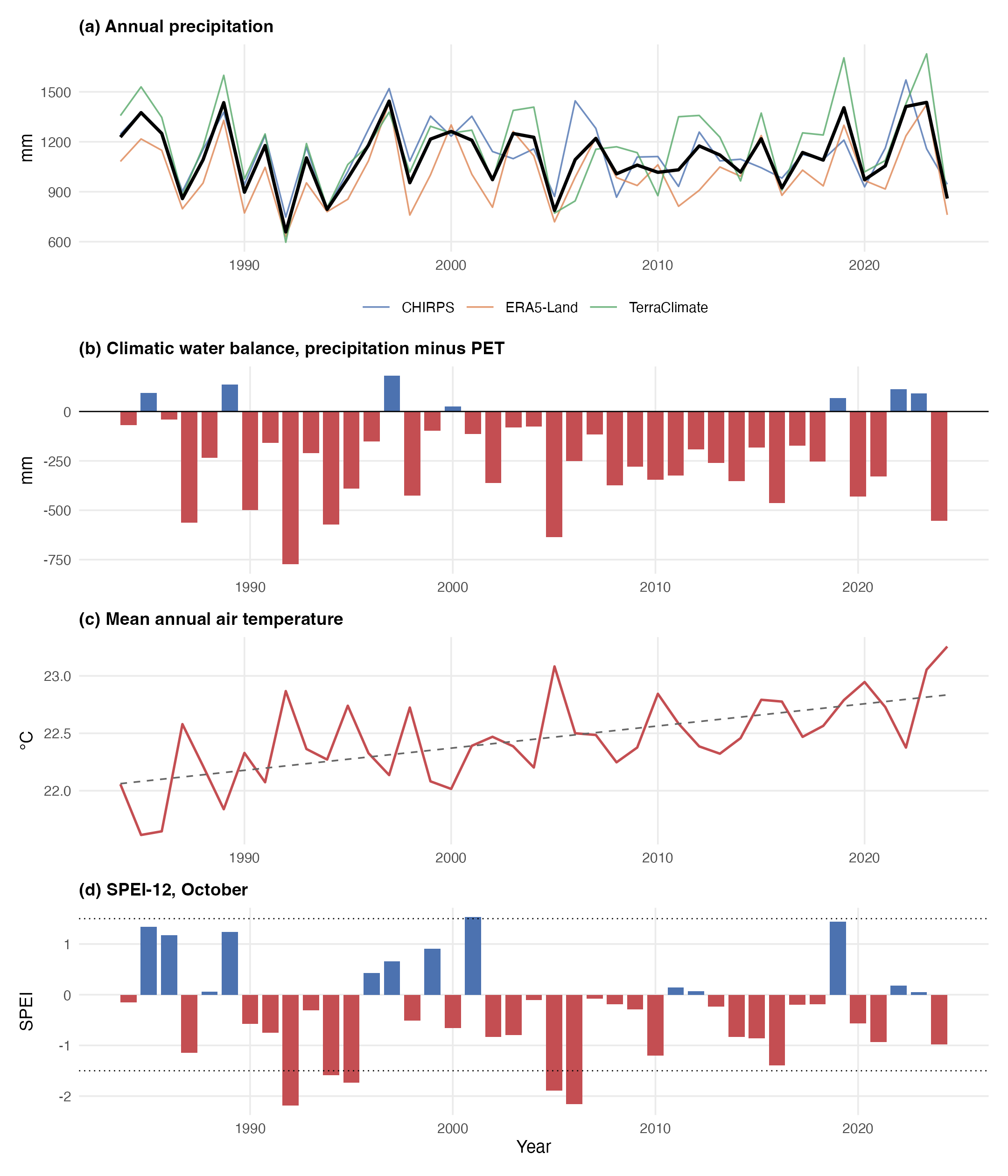---```{r}#| label: setup#| include: falsehere::i_am("chapters/01-introduction.qmd")source(here::here('05.scripts', '_common.R'))```Wetlands cover between 3% and 8% of the Earth's land surface and provide ecosystem services disproportionate to their extent: flood attenuation, water quality improvement, carbon sequestration, and biodiversity support (Mitsch and Gosselink, 2015; Davidson, 2014). Despite this, most countries lack comprehensive wetland inventories. Existing maps are fragmented, produced at incompatible scales with inconsistent methods, and rarely updated to reflect the dynamic character of wetland systems (Finlayson et al., 2018; Mahdianpari et al., 2019). In sub-Saharan Africa, the problem is acute. Many wetlands of continental significance function with limited mapping, and those that exist rely on single-date optical imagery that captures a snapshot rather than the seasonal and inter-annual variability that defines wetland function (Rebelo et al., 2009; Muro et al., 2016).Remote sensing offers the spatial and temporal coverage that field surveys cannot match, and two decades of methodological development have produced a substantial toolkit for wetland mapping (Ozesmi and Bauer, 2002; Mahdavi et al., 2018). Yet accurate mapping of inland wetlands remains difficult. Shallow, turbid waters confound optical classification. Cloud cover obscures tropical wet seasons precisely when inundation is greatest. Emergent vegetation masks the water beneath it. Coloured dissolved organic matter, suspended sediment, and phytoplankton blooms alter spectral properties in ways that atmospheric correction algorithms handle poorly (Matthews, 2011; Ogashawara et al., 2017). Higher-resolution sensors introduce their own constraints in spectral coverage, radiometric sensitivity, and temporal frequency (Palmer et al., 2015; Kutser, 2012).The concurrent availability of Sentinel-1 SAR and Sentinel-2 optical data since 2014, combined with the multi-decadal Landsat archive made freely available since 2008, now provides an unprecedented opportunity to address these limitations through multi-sensor time series analysis. Cloud computing platforms, particularly Google Earth Engine (GEE), have removed the computational barriers that previously made processing such large volumes of satellite imagery infeasible on conventional systems (Gorelick et al., 2017; Mahdianpari et al., 2019). These advances enable on-demand, large-scale wetland mapping that was not possible a decade ago.Endorheic watersheds in Africa present a further challenge that is not merely technical but social. Their ecological and economic significance is mediated by human populations whose livelihoods track the water. Remote sensing provides essential spatial data (Eva and Lambin, 2000; Philippe and Karume, 2019), yet it captures neither the adaptive strategies of local resource users nor the political ecology that governs access to fluctuating resources (Yiran et al., 2012; Sulieman and Ahmed, 2013; Demichelis et al., 2023). Maps that are technically defensible remain ecologically and socially incomplete.The spatial unit of this study is the basin, a term whose precise hydrological meaning the lake at its centre tends to obscure. A drainage basin, equivalently a catchment or watershed, is the whole area that drains to a common outlet, bounded by topography rather than by any water body within it. In an endorheic basin that outlet is internal: no channel reaches the sea, and water leaves only by evaporation and seepage from the terminal lakes and swamps where drainage gathers (Wang et al., 2018). Closed basins of this kind cover close to a fifth of the continental land surface, concentrate in arid and semi-arid regions, and are losing water storage worldwide (Wang et al., 2018). Lake Chilwa lies at the floor of one, a transboundary catchment of roughly 8,300 km² shared between Malawi and Mozambique (Kambombe et al., 2023), which we delineate from the terrain rather than adopt from a published product (Section 2.2.A).This distinction is the axis of the measurement, not a nicety of vocabulary. The basin is fixed; its divide does not move with the seasons. The water within it is not: open water advances and retreats across the flat basin floor through cycles of recession and refilling, and in the severest recessions the lake all but vanishes (Kalk, 1979; Njaya et al., 2011). The lake with its fringing Typha swamp and seasonal marsh forms a wetland complex of some 2,300 km², itself a small and shifting fraction of the catchment, and open water is a smaller and more variable fraction still. Separating that fluctuating extent from the fixed frame that contains it is the primary objective of this study. An inundation fraction means little without the reference area it is measured against, so we hold the catchment as the analytical boundary and treat the wetland complex and the open water as the quantities that vary within it (Pekel et al., 2016; Halabisky et al., 2016).This study addresses both limitations simultaneously. We combine multi-sensor remote sensing with sustained ethnographic fieldwork to map inundation dynamics in the Lake Chilwa Basin, one of Africa's most productive and volatile endorheic systems. The remote sensing component evaluates optical water-extraction indices against SAR-derived water maps, processed through a Google Earth Engine pipeline, to quantify what each sensor family detects and what it misses. The ethnographic component, conducted over 18 months across three districts, validates the satellite-derived classifications and reveals the social and institutional structures that determine how the lake's resources are governed, contested, and used.We read Lake Chilwa as a socio-hydrological system in the sense of Sivapalan and colleagues: a coupled human-water system whose lake dynamics and fishing society co-evolve through two-way feedback rather than through one-way climatic forcing (Blair and Buytaert, 2016; Xia et al., 2022). Mapping the inundation history and the fisher response that together constitute that coupling is the work of this paper, and it lays the empirical foundation for a coupled socio-hydrological model of the water-society feedback in the basin. That model is the central aim of the wider research programme, specified here and built on the record this study assembles rather than run within it (Srinivasan et al., 2017).## 1.1 Optical Index LimitationsWater-extraction indices derived from multispectral imagery are the standard tools for mapping surface water extent. Each exploits a different combination of spectral bands to distinguish water from land, but each fails under specific conditions that Lake Chilwa routinely presents.The Normalized Difference Water Index (NDWI; McFeeters, 1996) uses the ratio of green to near-infrared reflectance to delineate open water. It performs well where water is deep and clear (Ji et al., 2009) but struggles in shallow, turbid conditions because suspended sediment raises NIR reflectance, compressing index values toward zero (Xu, 2006; Li et al., 2013). In vegetated wetlands, vegetation reflectance dominates both bands and the index cannot distinguish water beneath emergent vegetation from surrounding marshland (Ozesmi and Bauer, 2002). Endorheic lakes with fluctuating shorelines present mixed pixels at the land-water boundary where NDWI thresholds systematically misclassify wet soil as dry land (Deus and Gloaguen, 2013).The Modified NDWI (MNDWI; Xu, 2006) substitutes shortwave infrared for NIR, suppressing the confusion between water and built-up or bare-soil surfaces that afflicts NDWI. It performs better in turbid and sediment-laden water (Li et al., 2013; Acharya et al., 2018) and is the strongest single optical index for the conditions this study addresses. It still fails beneath emergent vegetation, where macrophyte reflectance drives values negative even where standing water persists (Amani et al., 2020). In saline and endorheic systems, dissolved salts and algal blooms shift MNDWI thresholds unpredictably, requiring adaptive or Otsu-based methods (Pekel et al., 2016). Heimhuber et al. (2018) found that MNDWI required SAR fusion to map water extent beneath vegetation in the Murray-Darling system.The Automated Water Extraction Index (AWEIsh; Feyisa et al., 2014) combines five bands to suppress shadow and dark-surface commission errors. Its multi-band formulation captures contrasts that two-band indices cannot resolve, but subpixel mixing of emergent vegetation and water still reduces values below detection thresholds (Ji et al., 2015). Fisher et al. (2016) found that no single index, AWEIsh included, consistently mapped shallow or seasonal water bodies in a global comparison. In endorheic systems, AWEIsh can misclassify exposed lakebed and brine as water (Pekel et al., 2016).The Water Ratio Index (WRI; Shen and Li, 2010) uses the ratio of visible to infrared bands, yielding values above 1.0 for water. It suppresses cloud and shadow noise effectively (Li et al., 2023) and has shown strong performance in bare-soil landscapes in Ethiopia (Demelash et al., 2025). But where water, vegetation, and sediment share a pixel, the visible-band numerator inflates from non-water reflectance. The red band is particularly vulnerable to suspended sediment, which raises its reflectance sharply in turbid conditions. WRI has not been applied to endorheic or fluctuating lake systems.The Normalized Difference Pond Index (NDPI; Lacaux et al., 2007) was designed in and for semi-arid Africa, using SPOT-5 imagery to classify temporary ponds in Senegal's Ferlo region. It exploits the SWIR absorption of water against green vegetation reflectance, making it sensitive to the water-vegetation boundary where other indices fail. Campos et al. (2012) confirmed that SWIR-based indices outperform NIR-based ones for ephemeral ponds in the Sahel. NDPI is the algebraic inverse of MNDWI, carrying identical spectral information with reversed sign convention. It performs best on small, shallow, vegetated water bodies and loses sensitivity in deep or highly turbid water.The pattern across all five indices is consistent: each occupies a spectral niche but fails at the boundaries that define Lake Chilwa's hydrology. Shallow turbid water, vegetated wetland margins, fluctuating shorelines, and mixed pixels at the land-water transition are precisely the conditions where optical classification underperforms. These are also the zones of greatest ecological and socio-economic significance.## 1.2 Flooded Vegetation SignaturesThe unresolved problem in wetland inundation mapping is not the detection of open water but the detection of water standing beneath vegetation. Open water is spectrally and radiometrically distinct and has been mapped operationally for decades. Water held within an emergent macrophyte stand is neither, and the failure to resolve it propagates directly into every hydrological quantity derived from the map: inundated area, hydroperiod, and the timing and magnitude of recession and refilling. Tsyganskaya et al. (2018), reviewing 128 studies devoted to this single problem, state the position plainly: "In contrast to open flood surfaces, there is little research on the detection of flooded areas underneath vegetation. However, the disregard of FV can lead to an underestimation of the extent of an inundation." Six years later Amitrano et al. (2024) still describe flooding beneath the vegetation as "a less explored challenge" and warn that "the presence of vegetation may lead to an underestimation of the extent of inundated areas."Optical sensors cannot solve it, and the reason is physical rather than methodological. Mahdavi et al. (2018) put the limit categorically: "the penetration depth of optical sensors is so low that detection of the water beneath trees/dense vegetation is not possible." Adam et al. (2010) explain why the vegetation above that water is itself hard to resolve, since the reflectance spectra of wetland vegetation "are often very similar and are combined with reflectance spectra of the underlying soil, hydrologic regime, and atmospheric vapour," a mixture that depresses reflectance most severely "in the near-to mid-infrared regions where water absorption is stronger," which is where every shortwave water index takes its signal. The consequence they draw is that methods proven on terrestrial vegetation do not transfer to wetlands. The gap is long-standing rather than newly discovered. Rundquist et al. (2001) named it a quarter of a century ago, concluding that "it has been virtually impossible to detect the presence of standing water or wet soils under a full canopy of emergent macrophytes," and placing "assessing the impact of water beneath the vegetation canopy" among the field's defining research needs. Gallant (2015) generalises the diagnosis: from a remote sensing perspective wetlands are a moving target, "representing more of a moisture regime than a cover type."Radar addresses the problem in principle and saturates in practice. The double-bounce return from a water surface and vertical plant stems is the physical basis for detection beneath the vegetation, but it is conditional on wavelength, polarisation, incidence angle, and standing biomass. Tsyganskaya et al. (2018) report that studies converge on saturation points "at which water beneath the canopy cannot be detected any longer," beyond which "volume scattering from the canopy completely superimposes the contribution of double bounce," and note a lower bound as well, since "if the emerging part of the plants becomes too small, no considerable double-bounce scattering can be produced." Polarisation matters as much as wavelength. Adeli et al. (2020) identify the specific weakness of the configuration this study inherits from Sentinel-1: vertical transmit "may not reach the water surface beneath the vegetation cover because of its vertical orientation," while Mahdianpari et al. (2020) find that "the HH polarized signal is better able to distinguish wetland vegetation from water under calm water conditions." Battaglia and Bourgeau-Chavez (2025) quantify the dependence for *Typha*, the genus that dominates the Chilwa swamp, measuring stems of roughly 1.6 cm diameter at 20 to 28 per square metre and 1.8 to 2.2 m tall, a structure within reach of C-, S-, and L-band alike; for the denser and finer-stemmed *Phragmites* of the same study, C-band "was not able to detect flooding beneath mature Phragmites stands in many cases." Their strongest result is that the answer depends on the instrument: flooded-vegetation area over one delta varied by 22 per cent across the three wavelengths on the same scene.The cost of the failure has been measured, and it falls on this class alone. Slagter et al. (2020), working in a South African coastal wetland with the same sensors and classifier family used here, report that "subcanopy flooding could not be detected with Sentinel-1's C-band sensors operating in VV/VH mode," and resolved the problem by removing the class: their headline accuracy of 88.5 per cent is stated for the case "when excluding high-vegetated areas." Within their retained classification, user's accuracy falls from 94.0 per cent on unvegetated flooded wetland to between 22 and 48 per cent on the three vegetated flooded classes. The pattern recurs wherever per-class figures are reported. Mahdianpari et al. (2019) resolved shallow water and every non-wetland class above 90 per cent producer's accuracy but reached only 78 per cent for marsh and 70 per cent for swamp. Chasmer et al. (2020) synthesised 205 field-validated comparisons and found wetland form and type mapped at an average of 55 per cent accuracy from imagery of 11 to 30 m resolution, against 80 per cent at finer resolution. In semi-arid African settings the errors concentrate at the same boundary: Gxokwe et al. (2020) record omission errors of about 30 per cent in which water was confused with mudflat and emergent vegetation, "located at the interface of mudflats and other classes."The African record shows the same gap in a sharper form, because the region's large wetlands are dominated by the class that cannot be measured. On Lake Chad, the closest hydrological analogue to Chilwa, Pham-Duc et al. (2020) state the choice and its consequence explicitly: "In this study, we only consider open water bodies as surface water, whereas, in previous studies, water under vegetation was included as surface water." Counting the vegetated area as inundated moves the reported October 2013 extent to 12,800 km², against an open-water maximum of about 5,800 km² over the preceding two decades, so the definition alone shifts the number by roughly a factor of two, and the lake's permanent vegetation cover has itself grown from about 3,800 to 5,200 km² since the 2000s. In the Sudd, Rebelo et al. (2012) mapped open water and flooded vegetation separately across five dates and found flooded vegetation to be the larger component every time, between 63 and 86 per cent of total mapped wetland, while conceding that "the exact figures require validation against ground-based measurements" that the wetland's inaccessibility precluded. Validation is the recurring casualty. On the Kafue Flats, Aduah and Mantey (2012) report that "accuracy assessment of the derived maps was not conducted since ground truth data at the time of satellite over pass was not available," and attribute their success to the scarcity of the difficult class, since the tall *Typha* and *Papyrus* stands "cover a small percentage of the study area" and the dominant short grasses submerge completely. That condition is the inverse of Lake Chilwa, where the *Typha* fringe is the wetland. Schlaffer et al. (2016) mapped persistently and seasonally flooded vegetation across Zambia and reported no accuracy figure for any class. Where flood-exposure classes are validated, they are the weakest: in the Barotse Floodplain, Del Rio et al. (2018) achieved perfect user's accuracy on forest and upland eco-types while their wet and dry floodplain class fell to 0.64 producer's accuracy and their water class to 0.75 user's accuracy on four reference pixels. Gxokwe et al. (2020) note that few such studies exist in sub-Saharan Africa at all. Where a southern African floodplain has been mapped with the vegetated class retained, its share is decisive: Hardy et al. (2019), working the Barotse Floodplain of the upper Zambezi, report that "70% of the total water extent mapped was attributed to vegetated water, highlighting the importance of mapping both open and vegetated water bodies for surface water mapping."For a shallow endorheic basin the consequence is not a marginal error but a misreading of the hydrology. Where a lake recedes across a flat floor, emergent macrophytes colonise the exposed margin, so open water contracts while vegetated water expands, and a record built on open water alone reports desiccation where the wetland has in fact reorganised. Oakes et al. (2023), mapping the Barotseland Floodplain of Zambia, measured the share directly and found that "inundated vegetation can account for over three-quarters of the total inundated area, yet widely used EO mapping approaches are limited to the detection of open water bodies," with inundated vegetation accounting for a mean 80 per cent of wet-season inundation; they concede that any method resting on C-band backscatter, theirs included, "will underestimate the extent of inundation." The proportions are of the same order wherever they have been measured against radar. Across the lowland Amazon at high water, Hess et al. (2015) found open water to account for 9 per cent of wetland area against 77 per cent woody vegetation and 14 per cent aquatic macrophytes, and concluded that global datasets from lower-resolution optical sensors "capture less than 25 %" of the wetland area they mapped. Schroeder et al. (2015) put the same contrast in areal terms over the central Amazon, where radar returned 25,400 km² of open water but 67,700 km² once flooded vegetation was included, and reported their own coarse-resolution product limited by "the inability to detect standing water bodies underneath closed forest canopies." At global scale the shortfall persists: Poulter et al. (2017) set ground-based wetland inventories at 8.2 to 10.1 Mkm² against remote-sensing surface water near 6.5 Mkm². Vegetation indices offer no way round this, because the vegetation response outlasts the water: Sims and Colloff (2012) found floodplain greenness elevated by up to 19 per cent for thirteen months after flood recession, so greenness dates a past inundation rather than measuring a present one. The reviews converge on the same remedy, longer wavelengths combined with shorter ones, and on the same verdict, that it remains unproven. Poulter et al. (2017) recommend that "multi-platform remote sensing using both radar and optical observations are integrated at higher spatial resolution to resolve issues associated with low-detection probabilities in closed-forest canopy regions." The compilers of the standard global inventory reach the same conclusion from the other direction, noting that seasonal inundation driven by vegetation and saturated soils "are not as reliably mapped and contribute disproportionately to the large uncertainties in global wetland estimates," and naming among the field's outstanding needs "dependable estimates of soil surface moisture, sub-canopy inundation, refined topographic data and detection of hydrophytic vegetation" (Lehner et al., 2025). This study takes that remedy as its primary methodological objective, retaining the class that the state of the art excludes and measuring what its retention costs and recovers.The same gap runs through the hydrological models built on these maps. Global reach-scale reconstructions delineate their river networks from elevation and open-water layers (Yamazaki et al., 2019), then route water through channels (Lin et al., 2019; Song et al., 2025; Ji et al., 2025). A wetland enters such a network as a set of flow paths rather than as a store, so water standing within a reed stand for months is routed downstream in the model as it is passed over in the map. Calibration cannot correct what the structure omits, and in Africa there is little to calibrate against: Ji et al. (2025) report that their model could not reproduce observed runoff trends in the Niger or the Congo, attributing the failure to a paucity of training data. The measurement problem and the modelling problem are one. Both are limited by reference data rather than by method.## 1.3 SAR-Optical FusionSynthetic aperture radar addresses the specific failures of optical indices in inland wetlands. SAR operates at microwave frequencies, independent of cloud cover and solar illumination, two properties that make it indispensable for monitoring tropical wetlands where persistent cloud obscures optical sensors for months during the critical wet season (Mahdavi et al., 2018).Smooth open water produces near-specular reflection, returning very little backscatter to the sensor. C-band SAR typically records open water at -20 to -30 dB, well below surrounding land surfaces, enabling detection through simple thresholding (Martinis et al., 2015). Where vegetation stands in water, the signal follows a double-bounce pathway, reflecting from the water surface and then from vertical plant structures. This produces backscatter paradoxically higher than from the same vegetation when dry, because the smooth water surface enhances the coherent specular return (Hess et al., 1995; Tsyganskaya et al., 2018). The contrast between double-bounce returns from flooded vegetation and volume scattering from dry vegetation is the physical basis for detecting inundation beneath the vegetation.Sentinel-1, operational since 2014, provides C-band imagery at 10 m resolution with 6 to 12 day revisit. Its dual-polarisation mode (VV/VH) has been applied to wetland inundation mapping across diverse environments: the St. Lucia wetlands in South Africa (Clement et al., 2018), the Amazon lowlands (Hardy et al., 2019), the Okavango Delta (Luca et al., 2025), and seasonal lake cycles on the Tibetan Plateau (Zhang et al., 2019). Multi-temporal approaches exploit wet-dry season contrast to characterise hydroperiod without ground data. The Sentinel-1 Global Flood Monitoring service now processes all incoming acquisitions for near-real-time detection (Roth et al., 2025).C-band has limitations. Speckle noise degrades classification accuracy. Wind roughens water surfaces, raising backscatter above detection thresholds and causing false negatives (Martinis et al., 2015). Most critically, C-band's 5.6 cm wavelength cannot penetrate dense emergent vegetation such as Typha and Phragmites. Clement et al. (2018) reported poor classification in heavily vegetated zones. L-band SAR (approximately 23 cm wavelength), carried by ALOS PALSAR and the forthcoming NISAR mission, penetrates vegetation far more effectively. Hess et al. (2003) showed that L-band detected flooding beneath the vegetation at 50 cm depth in Amazonian floodplains, versus 80 cm for C-band.SAR interferometry offers additional capability. InSAR measures phase differences between acquisitions to detect centimetre-scale vertical displacement. In wetlands, the double-bounce mechanism preserves coherence, enabling water level change detection at resolutions exceeding gauge networks (Wdowinski et al., 2008; Hong and Wdowinski, 2017). Kim et al. (2021) mapped water level gradients across Tonle Sap at sub-monthly intervals. Temporal decorrelation and atmospheric phase delays limit the technique, particularly at C-band over intervals exceeding two weeks (Zebker and Villasenor, 1992). InSAR water level retrieval has not been attempted for African endorheic systems.Fusing SAR and optical data exploits their complementarity. Pixel-level stacking, decision-level fusion, and machine learning classifiers trained on combined feature spaces consistently outperform single-source models, with reported accuracies of 85 to 95 percent for wetland classes (Amani et al., 2019; Whyte et al., 2018). Xu et al. (2025) mapped surface water dynamics across East Africa at 10 m resolution by integrating Sentinel-1 and Sentinel-2 time series. Lubala et al. (2023) fused Sentinel-1, Sentinel-2, and ALOS PALSAR to map small inland wetlands in the Democratic Republic of Congo. These studies confirm that multi-sensor integration captures dynamics that either sensor family misses alone.#### Environment SetupA one-time Earth Engine setup adapted below from previous rgee workflows was render hidden. Run this chunk named `gee-setup-once` using `eval: true` in a fresh R session to build the project virtual environment. This will install the Earth Engine Python API into it, and authenticate. It does not run on render as cloned.```{r gee-setup-once}#| eval: false#| echo: false# ============================================================================# ONE-TIME Earth Engine setup. Run ONCE ONLY to configure a FRESH R session# (reticulate binds one Python per session). Venv kept at .venv/ rather# than the repo root; change ee_py to "./bin/python3" to match a root-level venv.# ============================================================================library(reticulate); library(rgee)# rgee::ee_install() builds a managed Python env at ~/.virtualenvs/rgee, installs# earthengine-api into it, and writes EARTHENGINE_PYTHON to .Renviron. Accept its# prompt to restart R; then re-run ee_Authenticate() and ee_Initialize().rgee::ee_install()rgee::ee_Authenticate()rgee::ee_Initialize(user ="seamusrobertmurphy", drive =TRUE, project ="murphys-deforisk")# --- OPTIONAL: Service Account Key for non-interactive / web renders + GCS ---# Guide: https://r-spatial.github.io/rgee/articles/rgee05.html# SaK_file <- "/path/to/SaK_rgee.json"# rgee::ee_utils_sak_copy(sakfile = SaK_file, users = "seamusrobertmurphy")# rgee::ee_Initialize(user = "seamusrobertmurphy", gcs = TRUE, drive = TRUE)``````{r}#| label: environment-setup#| comment: NA#| warning: false#| message: false#| error: false#| echo: true#| eval: falseeasypackages::packages("bslib","cols4all", "covr", "cowplot","dendextend", "digest","DiagrammeR","dtwclust", "downlit","e1071", "exactextractr","elevatr", "exifr","FNN", "future", "forestdata","gdalcubes", "gdalUtilities", "geojsonsf", "geos", "ggplot2", "ggstats","ggspatial", "ggmap", "ggplotify", "ggpubr", "ggrepel", "giscoR","hdf5r", "here", "httr", "httr2", "htmltools","jsonlite","kable", "kableExtrra", "kohonen","leaflet.providers", "leafem", "libgeos","luz","lwgeom", "leaflet", "leafgl","mapedit", "mapview", "maptiles", "methods", "mgcv","ncdf4", "nnet","openxlsx", "parallel", "plotly","randomForest", "rasterVis", "raster", "Rcpp", "RcppArmadillo","RcppCensSpatial","rayshader", "RcppEigen", "RcppParallel","RColorBrewer", "reactable", "reticulate", "rgee", "rgl", "rnaturalearth", "rsconnect","RStoolbox", "rts","s2", "sf", "scales", "sits","spdep", "stars", "stringr","supercells","terra", "testthat", "tidyverse", "tidyterra","tools","tmap", "tmaptools", "terrainr","xgboost",prompt = F)# Disable spherical geometrysf::sf_use_s2(use_s2 =FALSE)# Lift R's elapsed-time guard so long Earth Engine calls finish.setTimeLimit(cpu =Inf, elapsed =Inf)# Assign working directory to current locationknitr::opts_knit$set(root.dir = here::here())options(repos =c(CRAN ="https://cloud.r-project.org"),htmltools.dir.version =FALSE,htmltools.preserve.raw =FALSE)# Configure code formattingknitr::opts_chunk$set(echo =TRUE, message =FALSE, warning =FALSE,error =TRUE, comment =NA, # one cell error cannot abort the whole rendertidy.opts =list(width.cutoff =60))# --- Google Earth Engine via rgee (live init) ------------------------------# rgee::ee_install() saves EARTHENGINE_PYTHON (~/.virtualenvs/rgee) to .Renviron.# Bind reticulate to that same interpreter and set RETICULATE_PYTHON to match so# the two agree (no "request ignored" warning), then initialise.ee_py <-Sys.getenv("EARTHENGINE_PYTHON",unset =Sys.getenv("RETICULATE_PYTHON", "/opt/local/bin/python"))Sys.setenv(RETICULATE_PYTHON = ee_py)reticulate::use_python(ee_py, required =TRUE)library(rgee)rgee::ee_Initialize(user ="seamusrobertmurphy", drive =TRUE, project ="murphys-deforisk")# gcs = TRUE also works once a Service Account Key is configured (see above).# `ee` and rgee helpers (ee_as_sf, sf_as_ee, ee_extract, Map$addLayer) available.# Helpers to handle earth engine objects in tmap/leafletee_tile_url <-function(ee_image, vis_params) { ee_image$getMapId(vis_params)$tile_fetcher$url_format}ee_to_sf <-function(fc) {geojsonsf::geojson_sf( jsonlite::toJSON(fc$getInfo(), auto_unbox =TRUE))}``````{css, echo=FALSE, class.source = 'foldable'}div.column{ display: inline-block; vertical-align: top; width:50%;}#TOC::before { content:""; display: block; height:200px; width:200px; background-image:url('https://raw.githubusercontent.com/seamusrobertmurphy/mapping-wetland-inundation-lake-chilwa/refs/heads/main/assets/PNG/RADAR-render.png'); background-size: contain; background-position:50%50%; padding-top:80px !important; background-repeat: no-repeat;}```## 1.4 Study AreaLake Chilwa Basin is one of Africa's most productive endorheic systems, a transboundary catchment of roughly 8,300 km² draining the hills of southern Malawi and adjacent Mozambique to a terminal lake (Kambombe et al., 2023); the boundary we delineate from the terrain in Section 2.2.A encloses 8,752 km². At its floor the lake with its fringing Typha swamp and seasonally inundated marshland forms a shallow wetland complex of approximately 2,310 km², of which open water is a fluctuating share, on the order of a third in a wet year and far less during recession (Kalk, 1979). The lake was designated a Ramsar Wetland of International Importance in 1997, in recognition of its outstanding waterfowl populations and ecological significance (Wilson, 2007). The three surrounding districts, Zomba, Phalombe, and Machinga, support population densities of 162 persons km⁻² around the lake itself and considerably higher in the southern basin (Wilson, 2010), with 70 to 81% of households living below the poverty line and farming plots averaging 0.35 ha (Wilson, 2010). The fishery contributes on average 20% of Malawi's annual catch and in peak years has reached 43% (Chiotha, 1996; Njaya et al., 2011).The basin's hydrology is driven by unimodal rainfall (November to April) and sporadic chiperone rains (May to August). Annual fluctuations follow precipitation patterns closely (Ngongondo et al., 2011; Nicholson et al., 2014). Longer-term cycles of approximately 15 to 20 years produce dramatic lake recessions and varying degrees of complete desiccation (Kambombe et al., 2021). Wilson (2014) compiled the most complete chronology of lake levels, documenting major recessions in 1900, 1913-16, 1922, 1934, 1943, 1946, 1952, 1960, 1967-68, 1995, and 2012-13, set within a geological record of pluvial and inter-pluvial phases extending 450,000 years. Average maximum lake depth is 2.95 m; a prolonged dry phase between approximately 1760 and 1850 deposited a hard layer of homogeneous sandy clays at least 1.2 m thick that now underlies the lakebed (Wilson, 2014; Crossley et al., 1983). These fluctuations are not anomalies but the lake's defining ecological characteristic: a transient world that in some seasons supports a thriving fishery, a bustling marketing network, and burgeoning lakeshore settlements, while in the following season the shoreline may retreat by fifteen kilometres, leaving communities stranded from open water (Kalk, 1979; Allison and Mvula, 2002).During recession, the lake's three main commercial species, *Barbus paludinosus* (matemba), *Clarias gariepinus* (mlamba), and *Oreochromis shiranus chilwae* (chambo), take refuge in residual deep pools at alluvial river mouths and in swamps dominated by salt-hardy *Typha domingensis* Pers. (Howard-Williams and Walker, 1974; Howard-Williams and Gaudet, 1985). These species have evolved characteristics suited to a fluctuating environment: high fecundity, early reproductive maturity, broad diets, unspecialised spawning habits, and tolerance to wide environmental variation (Njaya, 2001). Refilling initiates complex succession dynamics, with emergent food webs driven by detritus and bacterial processes in alkaline, nutrient-rich sediments (Kalk and Schulten-Senden, 1977; Furse et al., 1979). Peak productivity reaches 159 kg ha⁻¹ (1979) and 113 kg ha⁻¹ (1990), surpassing Lake Malawi (40 kg ha⁻¹), Lake Tanganyika (90 kg ha⁻¹), and Lake Victoria (116 kg ha⁻¹) (Njaya et al., 2011; Vanden Bossche and Bernacsek, 1990). Wilson (2014) notes that the 1979 bumper harvest of 24,310 tonnes followed six years after the lake dried, during which oxidation of organic matter released nutrients that fuelled explosive productivity upon refilling.This boom-and-bust ecology sustains a complex mobile population. The basin's settlement history stretches back millennia, from Akafula hunter-gatherers through the 16th-century Maravi (Mang'anja) chieftancies, the mid-19th-century Yao migration from Mozambique, and the 20th-century Lomwe influx from Portuguese East Africa (Wilson, 2010). Today, permanent lakeshore communities of Yao, Nyanja, and Lomwe matrilineal descent groups farm the seasonally exposed lakebed and fish inshore waters. Seasonal migrants travel from as far as Machinga district to the north, spending weeks to months on zimbowera, floating platforms of piled Typha grass that serve as fishing camps in the lake interior (Murphy, 2014). These zimbowera neighbourhoods, such as Andere, Chambwalu, and Lingoni, support shifting populations of 300 to 1,000 fishers and sustain their own tea rooms, trading posts, and social governance structures. During the wet season, when fishing grounds are most productive but most inaccessible from the mainland, zimbowera cooperatives form along lines of village membership, kinship, and occupational specialisation. Seine-net crews of up to 80 fishers operate from large camps under single owners, while smaller gill-net cooperatives of three to four family members share boats, equipment, and risks on remote islands (Murphy, 2014). The fishery's principal port is Kachulu, on the western shore in Zomba district, which serves as the hub for a regional marketing network extending by bicycle and truck to Zomba, Blantyre, Liwonde, Phalombe, and Mulanje.The area of interest for all remote sensing analysis is the study's own basin polygon (`03.outputs/SHP/chilwa_basin.shp`), delineated by routing flow over a hydrologically conditioned digital elevation model rather than adopted from a public basin product. This replaces the hand-digitised outline of earlier drafts: the boundary is re-derivable from the elevation model itself by the flow-routing set out in Section 2.2.A, where a relief map of the basin also appears.## 1.5 Participatory Mapping DataThe reasoning behind multi-sensor fusion does not stop at the satellite. Optical indices fail in shallow turbid water and beneath emergent vegetation; SAR recovers much of what they miss yet cannot itself penetrate dense Typha. Each sensor earns its place by measuring a dimension the others cannot, and classification accuracy climbs as complementary sources accumulate: in a comparable Ghanaian peatland, overall accuracy rose from 71% for radar alone to 94% for a stacked optical, SAR, and terrain feature space (Amoakoh et al., 2021). The gain comes from complementarity, not volume. A source that repeats what another already records adds nothing, and a redundant band can even degrade a classifier. Read this way, the knowledge held by Lake Chilwa's fishers is not a departure from the remote sensing method but its extension: another source, subject to the same test as any spectral band, admitted because it carries information no sensor registers.What that source supplies is what the satellite stack cannot reach. Radar and optical indices share a blind spot in the marsh interior, where water stands beneath the vegetation that defeats both (Clement et al., 2018). Fishers work that interior through the recession cycle and know where the water goes. Their knowledge also holds what no reflectance encodes: the demand placed on the wetland, the causes behind an observed change, and the culturally defined places that have no spectral signature (Hodbod et al., 2019). Integrating local observation with satellite data is the standard response to optically complex, access-limited waters, where in-situ knowledge is treated as a first-class complement rather than mere ground truth (Hestir and Dronova, 2023). We therefore treat participatory mapping as a data source within a multi-source paradigm, and ask of it what we ask of every other source: that it add what the others miss. Local knowledge enters remote sensing in two registers: as an independent check on a satellite classification, and as the response variable itself where the phenomenon has no stable spectral signature. Lateef et al. (2025) exemplify the first, cross-validating flood-damage maps in the Hadejia wetlands of northern Nigeria against farmer-reported loss to within nine percentage points; Woodward et al. (2021) the second, deriving the very resource-use intensity classes their model predicts from participatory-mapped resource areas across a transboundary southern African landscape, where the contribution of Landsat spectra proved negligible.## 1.6 Research ObjectivesThis study pursues two aims. The first and primary aim is methodological. Surface water extent in vegetated wetlands is systematically underestimated, because it is mapped as open water. The two terms are used as though they were synonyms, so products that report surface water report only the fraction of it that lies open to the sky. Where flooded vegetation holds most of the standing water, as it does at Lake Chilwa, this is not a bias to be corrected at the margin but a measurement of the wrong quantity. We therefore measure surface water as the sum of open water and water standing within emergent vegetation, and we retain the vegetated class through every stage of the analysis rather than excluding it to protect the accuracy figures (Slagter et al., 2020). The obstacle is not the sensor alone. Water standing within a reed stand cannot be labelled from above at any resolution, and the marsh interior cannot be reached from the shore, so no conventional survey can supply the reference data the class requires. Fishers work that interior through the recession cycle and observe the standing water directly. Their observations are the training data this class has never had.The model we build on those labels combines four elements the literature has treated separately. It draws on harmonised multi-decadal optical reflectance and the five water-extraction indices computed from it (NDWI, MNDWI, AWEIsh, WRI, NDPI). It draws on radar backscatter at two wavelengths, Sentinel-1 C-band in VV and VH, which resolves open water and intra-annual timing, and ALOS PALSAR L-band in HH and HV, whose longer wavelength and horizontal transmit reach the water beneath the vegetation that C-band cannot (Adeli et al., 2020; Mahdianpari et al., 2020). It is fitted through spectral endmember mixture analysis, which resolves the water-and-vegetation mixture below the 30 m pixel as continuous fractions rather than forcing it wholly into one class or the other. And it is trained on participatory mapping with the basin's fishing communities, who work the marsh interior through the recession cycle and can report standing water within a reed stand that no overhead sensor and no image interpreter can observe. The basin boundary and drainage network on which the model is grounded are derived from the terrain by D-infinity flow routing (Tarboton 1997) over a depression-breached elevation model in WhiteboxTools and flowdem, rather than inherited from a public basin product. Under this aim we quantify the inundated footprint as the sum of open water and water held beneath emergent vegetation, rather than open water alone, and test whether the two components move together or compensate through the recession-refilling cycle. Three hypotheses follow, and each can fail.**H1.** Most of Lake Chilwa's surface water stands beneath aquatic vegetation rather than open to the sky. Total inundated area therefore cannot be recovered from open-water mapping, and existing surface-water records understate the basin's inundation by a large and measurable fraction. Leblanc et al. (2011) established this necessity for Lake Chad; Chilwa is the same class of shallow, vegetation-dominated lake.**H2.** No imagery-derived reference set can label the vegetated fraction: optical sensors observe only the skin surface of the vegetation, and C-band backscatter over water is continually modulated by wind roughening. Fisher-derived reference points supply labels for that class, and a classifier trained on them returns a flooded-vegetation extent that differs materially from one trained on image-interpreted or global-product reference data.**H3.** Vegetation activity remains elevated for weeks to months after water has receded, so index-based records date a past inundation rather than measuring a present one. Fisher observation registers recession as it happens, and the offset between the two records is therefore a property of the spectral response, not of revisit frequency. The second aim is to develop a socio-hydrological framework for watershed and natural-resource management in rural Africa: to test whether fisher knowledge supplies inundation and resource-use information absent from the satellite record, and whether coupling it with the hydrological record exposes a lake-fishery feedback that formal monitoring misses. Under this aim we validate the satellite-derived classifications against ethnographic data from key informant interviews, focus group discussions, and participatory mapping with migrant fishing communities, and document the fishing regulations, population movements, and resource-use patterns that formal monitoring frameworks have not captured. The coupled socio-hydrological model of that feedback is specified as the central next step of the research programme, not a claim of the present paper.------------------------------------------------------------------------
